隔壁的晚年生活

“来我寝室。牛二还是啤的?”

都快夜里一点了,隔壁寝室的“山哥”突然喊我喝酒,我不敢怠慢,披了件棉袄就过去了。推开门,三人已经围坐。

人们叫的“山哥”,满族钮咕噜氏,皮肤黝黑一口东北腔,在我们同学中年龄最长。听别人说是本科毕业在北京工作了几年,尝尽人间冷暖后考研回到了校园,读着硕士,做一些仪器方面的东西。以前跟女同学聊天,提到“山哥”她们都评价他人长得老实,憨厚,但我知道,他其实是胸口纹了一条龙的老江湖。

山哥招呼我坐下,递给我一小杯白酒。“来,走一个。”

一起碰杯的。山东大汉“黑总”,人生的白净,平日里爱抢红包,擅长讲授中南海野史和人情世故的规矩,对各企业灰色收入数额能信手拈来;还有一个个头矮小,满脸痘印的,人称“寝室长”,是今晚的主角,听说是感情生活遇到了空前的危机。

一口白酒闷下去,我开始自由落体,瘫坐在寝室长的床上,眯起了双眼。

“你和小璇到底是分手了还是没分?” 山哥质问寝室长。

寝室长嘬了一口酒,开始娓娓道来。小璇和寝室长恋爱从高中就谈起了,后来寝室长来北京读研,小璇也义无反顾跑到北京来工作。干了一年,可能是工作压力太大,现在听她家人的安排回成都工作去。

黑总听罢,食指对着寝室长点了几下,一副恨铁不成钢的样子。黑总也不客气,开始数落起寝室长来。“你说你,小璇来北京打拼,你天天打游戏。你读这个硕士挣多少?小璇挣多少?你就是个吃软饭的,小璇在你这儿哪里有安全感?”黑总喝了一口酒,歪着脑袋抬手指着寝室长鼻子说“我跟你说,小璇这一走你俩没戏!别指着她等你读完书,她现在已经到了谈婚论嫁的年龄了,你不急她和她家里急!”

寝室长极为丧气,耷拉这脑袋。面色通红,眼眶开始湿润,声音都有些颤抖 “你说的对,就像 S4 总决赛后[1] Faker 说的一样,输了就是输了,其他一切借口都没有用”

我噗嗤一声笑了出来,又赶紧用咳嗽搪塞了过去。“还有酒吗?” 我又是一口白酒,继续昏死过去。

“这事儿也不是没有办法” 山哥插了一句,寝室长眼里闪烁着希望。

“等小璇离职手续办好了,你别待学校了,好好陪她几天,找个好点的酒店缠绵缠绵,你懂的”山哥说。

“我是准备送送她” 寝室长似乎有些失望,又耷拉下了脑袋。

“哎呀,你咋不懂事儿呢” 山哥急切了起来,“你和小璇感情到了那一步,该上就得上了,一方面是给你们俩以后留个念想,再一个,她要是留了你的种,你俩这关系也就稳了” 山哥微微有些得意,点上了一支烟又接着讲,“我给你算算啊,你硕博五年,硕士完了就把证儿领了,今年或者明年,挑个好日子,到小璇家里去见见她父母,什么时候买房,以后回成都打拼,有些承诺要说出来,让她家父母知道你是有潜力有盼头的!”

听罢,寝室长突然崩溃了。眼泪在坑坑洼洼的脸上翻滚,波涛汹涌,诉说着郁结的愤懑和一个直男高尚的情愫。寝室长有些激动,端起酒杯又放下,“我算是想明白了!我这一辈子,一定要和小璇在一起”。

我坐立起来拍拍寝室长的肩膀,感受到了一个男人的炽热。拿起两个酒杯,碰了一下,递给寝室长一杯。自己又是一口,后来的事我就不知道了。

早晨醒来,我睡在寝室长的床上。懒得写了

注释:[1]《英雄联盟》2014赛季世界总决赛


Mac下LateX文字环绕图片宏包wrapfig的安装及使用

晚上写作业,无聊了没进展,怎么办,写日志。因为这是一件挺有意义也挺浪费时间的事儿。
你可能LaTeX代码敲得比我熟,哦;你可能用Tex Live Utility更新宏包,哦;你可能linux比我熟,哦;不打紧,这篇日志介绍一个不错的宏包,也记录一些操作细节,便于自己或别人重现,欢迎提建设性意见。

系统:OS X Yosemite 10.10.5
软件:XeTeX, Version 3.1415926-2.5-0.9999.3 (TeX Live 2013)
宏包下载:http://ctan.org/tex-archive/macros/latex/contrib/wrapfig/

使用的环境平易近人,和大多理工LaTeX使用者是一致的。
来,下面我们来手把手地做:

1# 下载宏包文件wrapfig.sty 并解压

2# 在Terminal中,复制宏包文件到制定目录
cd到你下载的目录/wrapfig/ 去(一般是/Download/啦)
cp -r wrapfig.sty /usr/local/texlive/2013/texmf-dist/tex/latex/base/

3# 刷新下LaTeX
sudo texhash
显示如下:
texhash: Updating /usr/local/texlive/2013/texmf-config/ls-R…
texhash: Updating /usr/local/texlive/2013/texmf-dist/ls-R…
texhash: Updating /usr/local/texlive/2013/texmf-var/ls-R…
texhash: Done.
就OK了

4#在你的论文中调用
\usepackage{wrapfig}

5#使用(含实例)
wrapfigure的用法:
\begin{wrapfigure}{行数}[位置][超出长度]{宽度}<图形>\end{wrapfigure}

实例:
\begin{wrapfigure}{l}{0.7\textwidth}
\includegraphics[width=0.65\textwidth]{placeholder}
\end{wrapfigure}

p29116337

Why do stars in pictures very often have four perfect beams?

Answer by Raziman T.V.:

These are Diffraction spikes.

The shared image was taken by the Hubble Space Telescope which is a reflecting telescope. Reflecting telescopes have a secondary mirror which stands right in the path of the incoming light.

Schematic of a Cassegrain telescope [1].

This is required to take the light collected by the primary mirror out of the telescope system where it can be read. But this creates a problem since the secondary mirror can’t clearly be floating in space. It is thus held in place using a support structure.

Support structure for the secondary mirror of a Newtonian eflector [2].

Light from strong point sources diffracts around the supporting structure, causing diffraction lines in the image which depend on the shape of the support arrangement.

Diffraction spikes produced by various support arrangements for the secondary mirror [3].

This is what happens with the Hubble images as well [4]:

The cross shape visible on bright objects (such as stars) in Hubble  images is a form of distortion that is visible in all telescopes that  use a mirror rather than a lens to focus light rays. The crosses, known  as diffraction spikes, are caused by the light’s path being disturbed  slightly as it passes by the cross-shaped struts that support the  telescope’s secondary mirror. It is only noticeable for bright  objects where a lot of light is concentrated on one spot, such as stars.  Darker, more spread-out objects like nebulae or galaxies do not show  visible levels of this distortion.

If you look closely, you can see that the lines emanating from the stars in the four directions are not of uniform intensity but show intensity oscillations typical of diffraction.

Sources
[1] Source: Wikimedia Commons. Author: Krishnavedala. License: Creative Commons Attribution-Share Alike 4.0 International
[2] Source: Wikimedia Commons. Author: SvonHalenbach. License: Creative Commons Attribution-Share Alike 3.0 Unported
[3] Source: Wikimedia Commons. Author: Cmglee. License: Creative Commons Attribution-Share Alike 3.0 Unported
[4] FAQ – Frequently Asked Questions. Hubble Europeans Space Agency Information Centre

Why do stars in pictures very often have four perfect beams?

Nutron Star free-precession simulation | MATLAB

Source code in MATLAB

clf
R=1000;r=1;phi=45;theta=5;omega1=1;omega2=0.023;
%%%phi/theta are inclination of precession
%%%and self_rotation respectively, omega1/2 are angular velocity of
%%%self_rotation and free_precession respectively
x=@(t)(R+r*cosd(phi)*sind(theta))*cosd(omega2*t)+r*sind(phi)*cosd(omega1*t)*cosd(theta);
y=@(t)(R+r*cosd(phi)*sind(theta))*sind(omega2*t)+r*sind(phi)*sind(omega1*t);
z=@(t)r*cosd(phi)*cosd(theta)-r*sind(phi)*sind(theta)*cosd(omega1*t);
ezplot3(x,y,z,[0,1000],'animate')

The simulation result

CB908695-967C-4A0E-88C3-8664F4745AF9

The problems merit further research

  1. what’s the relationship between precession radius R and the profile of binary system?
  2. How to demodulate this signal with free-procession by HHT analysis?
  3. For specific value of parameters, the signal has been found a drift of peak, does it have something to do with QPO?

Presentation on mode-mixing problem of EEMD | scripting only :D

Introduction

This is a work log of my recent research on Hilbert-Huang Transform [HHT], only part of it. Due to the fact that I was lazy about blogging, so the complete work log for HHT is not on the schedule of posting. This post is mainly about the mode mixing problems, including the questions of what it is, how it should be solved, and so forth.

Mode-Mixing Problem

As the essential purpose of Empirical Mode Decomposition [EMD] method is to decompose the signal to many IMFs with different range of frequency. From low frequency to high frequency, we can designate them as different mode. So if the situation occurs, that the frequencies in different range mixed in one signal or in one IMF, this is called the mode mixing problem. In this case we need a process to pick the specific mode or say to separate the different mode. It should be mentioned that the basic EMD method fails in this problem for some reason which I’m not gonna describe here.

Ensemble Empirical Method Decomposition [EEMD]

In 2009, Huang propose a method to solve the mode-mixing problem by adding white noise to the target signal. With the relatively high frequency white noise added, the proposed EEMD is developed as follows¹:

  1. add a white noise series to the targeted data;
  2. decompose the data with added white noise into IMFs;
  3. repeat step 1 and step 2 again and again, but with different white noise series each time; and
  4. obtain the (ensemble) means of corresponding IMFs of the decompositions as the final result.

well, it should be noticed that you add white noise once, you do the EMD then, you only get a series of IMFs with white noise you added. As step 3 and step 4 proposed, we need to repeat process of adding white noise and doing EMD, we obtain many different series of IMFs then, the amount of series depends on the ensemble number you set. Ensemble number means how many times you added the noise to the data. When you calculating the means of corresponding IMFs, the lager ensemble number you set, you can wipe the noise from the signal completely. As showed in these figures, with more times I added white noise, the signal here is outstanding from the white noise. In this case, the expected signal appears. Nevertheless, in the process of EEMD, the white noise or say noise, are not possible to exclude completely. So in practical situation, we concerned about the signal-noise ratio [SNR].

As you see in this figure, with the ensemble number up to one thousand, the SNR is good enough for the physical analyses. the high frequency signal constrain in the middle of the whole interval, which is exactly the signal I’ve constructed. So in the process of decomposing the the signal, it’s important to distinguish the signal with physical meaning from the noise. So the question here is Which components of a signal are noise?

Well, as the lower amplitude of the noise you added, the more significant the signal was. FYI the proper low amplitude of noise can raise the SNR. By setting different amplitude (different means statistical expectation different, due to that the white noise added by random numbers varies by an expectation, amplitude of noise are different in each noise-added process of course.) the specific components of the signal had distinct decrease for same ensemble number. Bang! That’s noise for sure! Because, obviously the signal only agree to the mean value when the ensemble number increase.

Does it mean you can add unlimited low noise to the signal to obtain best SNR? Absolutely not! The fact is that if the added noise amplitude is too small, it may not introduce the change of extrema the EMD relies on somehow¹. So here is the STRATEGY of adding white noise: add the amplitude 0.2 times the standard deviation of the original signal, and set the ensemble numbers large enough for acceptable SNR, which I recommend 1000 times at least.

Last but not least, I post two decomposition result of EMD and EEMD for comparison as follows:

left:EMD mode-mixing result; right:EEMD mode-mixing (solved) result
EMDsimulationEEMDsimulation

Reference

  1. Ensemble empirical mode decomposition: a noise-assisted data analysis method. Advances in adaptive data analysis, 1(01), 1-41.

A Review of calculating Energy flux for HXMT | Physics background in a nutshell

Abstract: HXMT, Hard X-ray Modulation Telescope is the project I’ve been working on. The major purpose in this period is to calculation the energy flux of instruments on satellite. My last work log introduced the numerical calculation tool of my work, Mathematica, which maybe not as elegant and cool as what c++ or python does, but it turns out that works at all. This log mainly focused on the relevant physics stuff concerned in this work, which contained spectral model of astro-sources, interstellar absorption model, effective area of instrument.

RADIATIVE PROCESSES IN ASTROPHYSICS

As my last log mentioned, approximately half of my work first focused on the INTEGRAL catalog. obviously, the first thing before calculating the HXMT energy flux is verify the method and spectral model are trustworthy. Well, the INTEGRAL provided the general reference catalog, of which I used version 39. In the catalog, there are 4 columns reported the value of calibration energy flux calculated by XSPEC. (It’s a good idea to post some logs of XSPEC) So, the first step is to calculate the flux in 10-50KeV, 20-60KeV, 60-200KeV with the model parameters given by the site: http://isdc.unige.ch/integral/catalog/39/catalog.html The reported calibration value are given in unit of cgs, so the energy fluxes are in unit of erg\cdot cm^{-2}\cdot s^{-1}, so the flux expression are given by:

\int{\frac{A}{6.24\times {{10}^{8}}(KeV\cdot er{{g}^{-1}})}\cdot E\cdot {{E}^{-\Gamma }}dE}

\int{\frac{A}{6.24\times {{10}^{8}}(KeV\cdot er{{g}^{-1}})}\cdot exp(-E/{{E}_{cut}})\cdot E\cdot {{E}^{-\Gamma }}dE}

those two equation calculated the powerlaw model and cutoff model, in which A refers to normalization coefficient  and \Gamma is photon index. Oops! My logic is a little bit chaotic right now, I should have introduce all the spectral models before calculating the flux utilizing those models. Anyway I’m not tend to list the mathematical expression of powerlaw, high energy cutoff, broken powerlaw, power. 

INTERSTELLAR ABSORPTION

In the content above I didn’t mention that calibration value includes a energy range 3-10KeV, in which energy range the photon is call soft X-ray radiation. The extragalactic radiation of X-ray is dominated by soft X-ray radiation. As the interstellar molecule have the property to absorb the radiation, the soft X-ray radiation must consider interstellar absorption effect.

f(E)=f_{0}(E)e^{-\sigma(E)n_{H}}

where\sigma(E) 
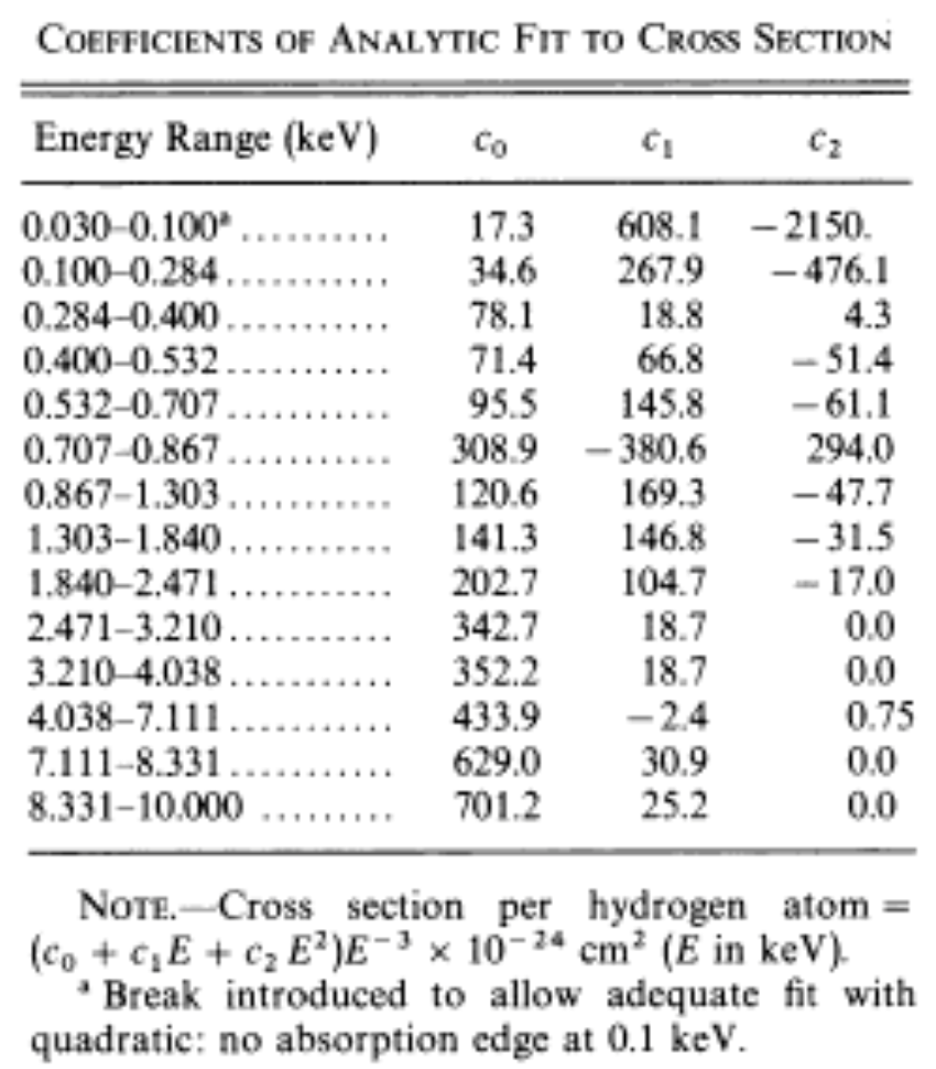
is the interstellar medium cross-section.

there are many version of cross section, but INTEGRAL catalog utilizes Wisconsin Cross-section:

\sigma (E)=({{c}_{0}}+{{c}_{1}}E+{{c}_{2}}{{E}^{2}}){{E}^{-3}}\times ({{10}^{-24}}c{{m}^{2}})

and the coefficients of analytic fit to cross section are given in following table:

Screen Shot 2015-03-12 at 8.49.12 AM

As we can see, the interstellar absorption only happened under the energy of 10KeV. So we can transfer the integration to the following form:

\sum\limits_{i}{\int\limits_{i}{\exp [-({{c}_{0}}+{{c}_{1}}E+{{c}_{2}}{{E}^{2}}){{E}^{-3}}\cdot {{10}^{-24}}\cdot {{n}_{H}}\cdot Af(E)dE}}

Though this log was aimed to introduce the physics regime, but it occurred to me to verifying the reason that Mathematica results had the deviation to XSPEC while considering the interstellar absorption which you have to carry out the numerical integration. So I utilized Python to set a parameter, energy bin, which is the same thing to interval. This parameter partitions the flux range to N sub-intervals.

and here’s the python code:

import numpy as np
import pylab as pl
import scipy
A=10 #normalization coefficient 
nh=0.26 #column density of hydrogen(unit of 10**22atom/cm**2)
c=2.1 #photon index
N=20000 #energy bin=N
x1=np.linspace(3,3.21,N,endpoint=False)
y1=np.trapz(np.e**(-(342.7+18.7*x1+0*(x1**2))*(x1**(-3))*(10**(-24))*nh)*A/(6.24*(10**8))*x1*(x1**(-c)),x1)
x2=np.linspace(3.21,4.038,N,endpoint=False)
y2=np.trapz(np.e**(-(352.2+18.7*x2+0*(x2**2))*(x2**(-3))*(10**(-24))*nh)*A/(6.24*(10**8))*x2*(x2**(-c)),x2)
x3=np.linspace(4.038,7.111,N,endpoint=False)
y3=np.trapz(np.e**(-(433.9+(-2.4)*x3+0.75*(x3**2))*(x3**(-3))*(10**(-24))*nh)*A/(6.24*(10**8))*x3*(x3**(-c)),x3)
x4=np.linspace(7.111,8.331,N,endpoint=False)
y4=np.trapz(np.e**(-(629+30.9*x4+0*(x4**2))*(x4**(-3))*(10**(-24))*nh)*A/(6.24*(10**8))*x4*(x4**(-c)),x4)
x5=np.linspace(8.331,10,N,endpoint=False)
y5=np.trapz(np.e**(-(701.2+25.2*x5+0*(x5**2))*(x5**(-3))*(10**(-24))*nh)*A/(6.24*(10**8))*x5*(x5**(-c)),x5)
flux=y1+y2+y3+y4+y5 #unit of erg/cm^2/s
print flux

It turns out that XSPEC utilizes N\approx 120 and Mathematica’s N\geqslant 10000

INSTRUMENT EFFECTIVE AREA

Instruments have different matrix responses for different photons in various energy. Till now we have considered the interstellar absorption, spectral and here’s another parameter we should integrate with, that is instrument effective area.

{D}=P(E) \times F(E)

where D is observed value, F is the spectrum we knew, P is the matrix responses. For flux we care about, we can calculate the integration:

{flux}=\int{\text{area of instrument}\cdot \sigma{(E)}\cdot{f}(E)dE}

 integral-effective-area


Those three aspects are in priority list of my recent work, I’ve introduce the basic physics behind it. For more information of HXMT, please visit the site: www.hxmt.cn

一包充满着乡愁的“芙蓉王”吸完以后,到学校的小卖部想充值一下乡愁,惊讶地发现帝都小卖部不售“芙蓉王”。索性咬咬牙买包24大洋的“云烟”,好歹也算在母校的初恋。但更让我惊讶的是,帝都的“紫云”竟然只卖10元。我不懂什么是市场经济,但这就是市场。

Mathematica | A brief log of my recent work

“Calculation of energy flux in High energy Satellite” is my recently work on INTEGRAL catalog. My goal is to calibrate the emitting model and the interstellar absorption model in X-ray energy range. While the model is convincing, I can boldly utilize those models on HXMT catalog for estimation. The following notes are focused on Mathematica which I used to produce the data analysis.

  • Data Import/Export

Mathematica can read many types of data file, like .txt .dat .fits (It’s ok for read, but normally the capacity of  FITS file are about 10MB, so it’s not ok for program running with such a huge burden), especially for large group of data analysis, this proper of mathematica is very useful. When talked about the fits file, there is a little trick I want to note down that I can use the Export function in fv tool to export the specific rows and columns with .txt for data analysis, instead of running the whole FITS raw data. Here’s the code for Importing files:

Import["complete path of your file","Table"]

I import data as table like {{1,2},{44,63}}. What is important to notice is the path syntax. For example, my OS X system have to start with a slash”/” and end up with file name, NO slash in the end.

eg. Import[“/Users/tuoyouli/Desktop/data.txt”,”Table”]

What’s next is exporting file which is similar with Import syntax.

Export["complete write path",data,"Table"]
eg. Export["/Users/tuoyouli/Desktop/HXMT flux/HEcounts.dat",Table[{b[[i]][[2]], b[[i]][[3]], a[[i]]}, {i, 1, Length[a]}], "Table"]
To explain this code let’s move to next section about reorganize data.
  • Data Regroup

The previous Export code include a data reorganize part:

Table[{b[[i]][[2]], b[[i]][[3]], a[[i]]}, {i, 1, Length[a]}]

while a,b are two-dimensional data group like {{1,2,1},{3,4,3},{5,6,5}}, the b[[i]][[2]] is a coordinate that can pick the specific element of the group b. And based on this, you can pick up the specific elements in different data group and then reorganize them by code Table in anyway you like. Huzzah! Another interesting normal usage about reorganization, is to combine two lists on plotting. When I want to plot how groupA depends on groupB, I can write down this code:

ListPlot[Transpose[{A,B}]]

of course, listA and listB must in same length.

  • Numerical Calculation(!)

For this section is the key function for Mathematica. I was told the somebody believe the Calculation Physics is the third fundamental part of physics, the other two are theoretical and experimental physics. Wow, that’s huge! Anyway here’s the numerical calculation which can give out the numerical results instead of analytical results. So when talk about Numerical, two things occur to me. One, numerical integration. Two, fitting and interpolation values. For numerical integration in Mathematica, I can simply use the code NIntegrate[], this code contains different numerical integrate method like Monte Carlo. (for more detail read on NIntegrate Method) Another stuff is interpolate value for a experimental separated data to a curve or line.

eg. Interpolation[data,InterpolationOrder->3,Method->Spline]

This a 3-order spline to interpolate the data, also there are plenty of numerical method for interpolation. (Read More)


So, perhaps in the following career I don’t have much chance to use Mathematica, because Matlab takes the lead, you don’t really want to use the different syntax with people around you. But Mathematica is so elegant and so easy to use, this work was based on Mathematica which help me get through all the obstacles. And this work log may at least not be nonsense.

“苏格拉底”在喧嚣中死亡

2013-07-27(文)

确实我敲打文字的次数不是很多,以至于1个小时过去了,我不断纠结和反复着开头,而迟迟没有敲键。也或许真的是脑中的片段过于琐碎,没有这个功力将其合理地串联起来。于是,我索性胡乱地草草开头,哪怕只能写到这里,也就罢了。

一. 过于喧嚣的孤独

真是可笑,这草草的第一段竟然让我找到了一个有趣的开始行文的话题。上文有一个词很奇怪,至少是我读的东西里几乎没有出现过。虽然是我杜撰的,但我却觉得是一个普遍的状态——敲键。现在人类的生活状态,工作状态和心理状态都发生了巨大的改变,这种变化在我看来,刚才那个文字上的一点点字义的变化对我产生了一个不小的笑点,但宏观到我能观察到的微观的小世界,这种深刻而剧烈的变化给我更多的是不安的恐惧。

不知从什么时候开始,发现自己越来越难以独处,一件事的意义 总要被一个或大或小的集体的背景所框定和绑架,其定义和理解往往受到一个或大或小的舆论的限定。无数次漫无目的地翻出手机检查一下消息栏,即使长期只有寥寥的中国移动的客服短信。而且总是有一种强迫症似的冲动去浏览未读信息。可笑的是,强迫症在当下也被标榜成为一种时尚,我不清楚人们是受到舆论的牵引如此病态和机械的,还是被时代标记了一种脸谱化的习惯。

为此,我曾长期逃避社交网络,逃避一切有大众舆论和自我袒露的地方。对于逃避大众舆论,一部分处于对 被思想 的担忧,但更主要是对其受群体心理规律支配的强大的不可逆性和排他性的恐惧。万一失足,挑战大众不仅艰辛和徒劳,更会被社会教化天衣无缝的“诡计”折磨的捶胸顿足、无可奈何。对于社交网络的自我坦露,我曾有过愤慨的谴责,在笔墨间骂他们是精神的婊子,信息的便捷传输使信息沦为纯粹的信息,如同计算机代码一般在人与人之间交互,然而却没有了灵气以及分量。

我想过写一点愤青檄文之类来阐明其病态,但是却不经意落入了一个可笑的悖论。在社交网络的语境下阐述社交网络的病态,如同醉酒之人说自己没醉一样的滑稽。而且哪怕是有人附和,这其中的矛盾也令人哭笑不得。赞同,是什么程度上的赞同?是同样冲破了悖论枷锁的义无反顾,或者是因为同样醉酒之人心灵的一点点契合,或是一瞬间朦胧的“有感觉”。我总是以“患不知人也”鼓励和安慰自己,然正是如此,哪怕是越来越不会独处,却真正越来越孤独,这孤独过于喧嚣罢了。

看到一些朋友发表一些文字一些图片,我努力去揣摩他们的心理状态,哪怕我能很敏感地洞察,但是奇怪的是我很难把他们反射到自己的心灵,因此有时我还双关地调侃自己是20世纪的人。这种隔阂如果按照孔子“不患人之不己知”的逻辑推己及人的话,那是多么可怕的一幅图景,人们不过是自说自话地按照生命的节律演着一出出舞台剧。我不愿意这样推断,我宁愿相信只是自己修为不够。但实际上并不是我个人的臆断就能改变现实图景的走势,我能感觉到和很多朋友甚至是亲人走得越来越远了,如果我孤高到你我想象中的程度那我也就没有恐惧了,但实际上我就是废柴一枚。

在交往人群的分类中,有一些奇怪的划分,老乡、同学这些划分依据就如同将数字按照高矮分类一样无聊。或许三天一条短信才算做是常联系,可能电话中你言我语滔滔不绝才算是有感情,但我一般低于这个标准,但我也仅仅是低于一个标准。一个未加约定就已经俗成的标准将生命里的几乎所有人不加区别的疏离,而这又仅仅是前提,真正的疏离被决定于我产生了这样的想法。

很自然地,群体情愫的伦理关怀将这样的个体视为弱势给予关注(哈),而对这种定位的强烈反感和排斥便不可避免地将我拽入一个极端,或者说是这种极端的态度将我塑造到了一个极端,排斥和人交往。甚至是上一秒还和人热络着,这一秒可能突然愣住发一小会儿呆,脑子里闪过无数次演绎过的消极得令人叹息的支离破碎的东西。

但如果兜一个圈又回到孔子的假设,那一切还是能看到乐观的一面,既是 这些令我不安的谈论自我的言语完全不必,我并没有悲剧性的历程,只不过我不勤于演戏、欺骗上帝、欺骗自己。

二.苏格拉底已死

但是不欺骗上帝,仅仅这样我就能是问心无愧的吗?

前两天和一高中同学争论,争论的问题的本身对我来说是不证自明的,但是哪怕我的论证字字句句掷地有声,但是面对他的诡辩或者严格说是小学生吵架的言语方式,我可以不屑他完全没有哲学素养,我可以表达震惊和不可理喻,但是我唯一不能做到的就是说服他。

诸如:XXX的言论只代表XXX他自己,我们世界有多少人,他才占到几分之几,根本没有代表性,你没有辩证地表述这个问题,说明你的言论是有漏洞的……以一种M16全自动步枪的节奏堆砌辞藻不断打断对方不断提高音量。显然是吵架而不是争论。

我放弃了,我没有再试图说服他,我想当然的认为他的幼稚和他获得真理的权利并不对等。我再次选择了逃避,逃避大众因为群体的愚蠢和无意识,这次则是一种“机智”。这种机智虽然不同于“大学生”群体的老练和圆滑,但是这种机智却使我一天天缩小自己满以为值得和可能交流的对象。苏格拉底已死。

选择背后的基础是勇气和责任,对于大众的逃避起码是勇气的缺失,苏格拉底没有如此选择,他用生命践行了他的哲学和他声称的神明所赋予给他的开导大众的责任。这是自主性同样是人性,更是华丽丽赤裸裸地对人性尊严的体现。我的怯懦不能证明怯懦自身是站不住脚的,即我们不去褒贬苏格拉底的诘问。但是却可以质疑,对于我的论证,到底是听者心灵没有敞开,还是我貌似高贵的知识不够有力?

讽刺的是,现在已经过12点了,也就是说今天是我的生日,而今天我却宣布了我一直视为偶像和导师的苏格拉底之死。

但是巧合的是,苏格拉底之死浇灌出了其哲学以及其崇敬者的信仰。