在服务器上使用GitHub的艰苦斗争

小白一个,想在服务器上实现Git的版本控制这么一件事情,折腾了很久。记录一下遇到的问题和解决:

git clone my repository

It turns out that

Connection timed out. Fatal: The remote end hung up unexpectedly.

This took 3 days to find out the possible solution. Yesterday, I was having a small talk to lab mate. I was asking “hey, is there any problem when we use hlogin host?” “Which one do you refer exactly?” “hlogin07“”That one is unable to wget or git

I was like …… SHIT!

so I changed it to @hlogin03.ihep.ac.cn. Well, clone process works fine now.

git push my update

after git add and git commit, I carry out git push origin master. Another error occurred

error: The requested URL returned error: 403 Forbidden while accessing https://github.com/tuoyl/hxmtanalysis.git/info/refs

fatal: HTTP request failed

So I checked what the heck is that 403 Forbidden stuff. And google feeds me back that this is due to some version problem. Yeah, of course, the Git version on the server is the old school version which they prefer, RollingMyEyes.

Anyway, there is another approach fixing it, remote my git with ssh instead of HTTP format(something like that).

So I run git remoter set-url ssh://git@github.com/tuoyl/hxmtanalysis.git, and git push again after it. Guess what, I don’t have an SSH key for this GitHub account. I really know nothing on this.

Add an SSH key associated with my account

An SSH key was generated on the server first:

ssh-keygen -t rsa -b 4096 -C “crazyuni1993@gmail.com”

add a key associated with my GitHub account, setting — SSH and GPG keys, which took me a while to find it.

copy the information within ~/.ssh/id_rsa to fill in the table when adding an SSH key on GitHub.

Well, you pretty much good to run! Cheers!

Deducing GJ electron density

Prove that plasma density surrounding Neutron Star follows:
\rho = \frac{\nabla\cdot \vec{E}}{4 \pi c}= \frac{-\vec{\Omega} \cdot \vec{B}}{2 \pi c }\frac{1}{1-(\Omega r/c)^2 \sin^2 \theta}
because the Lorentz force vanish here, we have:
\vec{E} = - \frac{\vec{\Omega}\times \vec{r} \times \vec{B}}{c}
So,
\frac{1}{4\pi} \nabla \cdot \vec{E} = - \frac{1}{4\pi} \nabla \cdot (\frac{\vec{\Omega}\times \vec{r} \times \vec{B}}{c}) = - \frac{1}{4\pi} \nabla \cdot [\frac{(\vec{\Omega}\times \vec{r}) \times \vec{B}}{c}]
make use of vector formulas, we obtain
\frac{1}{4\pi} \nabla \cdot \vec{E} = - \frac{1}{4\pi} \left\{ \vec{B} \cdot [ \nabla \times \frac{ \vec{\Omega} \times \vec{r}} {c}] - \frac{(\vec{\Omega}\times \vec{r})}{c} \cdot (\nabla \times \vec{B}) \right\}
due to the Maxwell’s equation \nabla \times \vec{B} = 4 \pi \vec{J} = 4 \pi q \vec{\beta_t} = \frac{\vec{\Omega} \times \vec{r}}{c} \cdot (\nabla \cdot \vec{E})
Thus,
\frac{1}{4\pi} \nabla \cdot \vec{E} = - \frac{1}{4\pi} \left\{ \vec{B} \cdot [ \nabla \times \frac{ \vec{\Omega} \times \vec{r}} {c}] - (\frac{\Omega r \sin \theta}{c}\vec{\phi}) (\frac{\Omega r \sin \theta}{c}(\nabla \cdot \vec{E})\vec{\phi}) \right\}

so,
[1-(\Omega r/c)^2 \sin^2 \theta] \frac{\nabla \cdot \vec{E} }{4 \pi} = - \frac{1}{4\pi} [\vec{B}\cdot(\nabla \times \frac{\Omega r \sin \theta}{c} \vec{\phi})]
where, \nabla \times \frac{\Omega r \sin \theta}{c} \vec{\phi} can be calculated by \nabla calculator as spherical coordinate form:

\nabla \times \frac{\Omega r \sin \theta}{c} \vec{\phi} = \frac{1}{r \sin \theta}[\frac{ \partial}{\partial \theta}(\sin \theta \frac{\Omega r \sin \theta}{c})- \frac{\partial 0 }{\partial \phi}] \vec{e_r} + \frac{1}{r}[\sin \theta \frac{\partial 0 }{\partial \phi} - \frac{\partial}{\partial r} ( r \frac{\Omega r \sin \theta}{c})]\vec{e_{\theta}} + \frac{1}{r}[\frac{\partial}{\partial r}(r 0) - \frac{\partial 0 }{\partial \theta}] \vec{e_{\phi}}
\nabla \times \frac{\Omega r \sin \theta}{c} \vec{\phi} = \frac{2\Omega \cos \theta}{c} \vec{e_r} - \frac{2 \Omega r \sin \theta}{c} \vec{e_{\theta}} 
\nabla \times \frac{\Omega r \sin \theta}{c} \vec{\phi} = \frac{2}{c} \vec{\Omega}
Therefore,
[1-(\Omega r/c)^2 \sin^2 \theta] \rho = - \frac{1}{4 \pi}(\vec{B} \cdot \frac{2}{c}\vec{\Omega})

finally, we obtain
\rho = \frac{-\vec{\Omega} \cdot \vec{B}}{2 \pi c }\frac{1}{1-(\Omega r/c)^2 \sin^2 \theta}

Fermi data analysis notes on Pulsar

The flux of quiescent state of Crab Nebular in a time interval of 360 days over a ten-year observation was obtained utilizing Fermi data. The fluxes of point sources in ROI (region of interest) are written in file *results.fits generated by Fermi tool gtlike .

The detail of analysis thread can be found here. However, there were problems not reported in the instruction.

1. Environmental variables

The source model XML file was generated by user donated Python script make3FGLxml.py. Before this process, the event data was selected, the counts map was generated, and the newest version of diffuse models was downloaded from Fermi website.

Because of some unknown glitches, the following steps are required to run make3FGLxml.py successfully:

after compiling Fermi environment by doing

$ fermiinit

$ which python

the path of Python compiler (I’m not sure how to call it) is set to ~/Documents/Fermi/ScienceTools-v10r0p5-fssc-20150518-x86_64-unknown-linux-gnu-libc2.19-10/x86_64-unknown-linux-gnu-libc2.19-10/bin/python

set a link for this path to the path of /usr/bin/python by doing:

$ ln ./python /usr/bin/python

By doing those processes, python script for generating source model XML file is ready to go.

2. Script input parameters

When running gtlike, a bizarre problem occurred: buffer overflow detected, and the process was terminated. We spent a lot of time debugging, and it turns out that the solution is to simplify the input parameters of running python script. I suggest running make3FGLxml.py in the path of point source file gll_psc_v16.fit. In this case, cut the absolute path of point source file to simplify the input parameters.

$ python make3FGLxml.py gll_psc_v16.fit …

3. Another Environmental variables problem

The last step of spectral fitting processes is to use HEASOFT tool farith to subtract model source counts map from observed counts map. The HEASOFT environment is required

$ heainit

Setting heainit environment when finishing all Fermi analysis processes, which includes gtselectgtmktime, gtbin, gtltcube, gtexpcube2, gtlike, gtmodel, is recommended.

前几天在微博上,看E和他们学校的官微较劲。官微在评论里使用了不当言论,E撕得不慌不忙,铿锵有力,最后对方是道歉了。而事儿还没完,第二天E跑到校长办公室反映了情况,得到了积极的回应。作为观众,看得挺过瘾的。

撕逼这事儿,你占了理,还撕得漂亮,那就是大快人心的大好事。涨粉

而我,生性可能比较软弱,撕逼撕得少,更多的时候是逃避冲突自己受委屈,剩下的情况就是上拳头揍人了。

但是我们家有外交强硬的基因,我看E在互联网上扇别人耳光时,经常想起我外公。虽然和外公疏离了,但是小时候过年回老家,还是听过一些故事。

外公生在我们老家湖南的农村,当时家里是地主。外公十几岁的时候,唯唯诺诺,还有些结巴。带着个瓜皮帽,脑袋上长了癣,因为痒,所以要时不时隔着帽子挠头。

去收租子这种与人打交道的事儿,他是不敢做的,但我外公的爸爸叫他去,他也不敢不去。十几岁的少爷,鼓起勇气,磕磕巴巴地喊“王……王老二……收……收钱”,喊完就躲到他几个表兄弟身后去了。这样的地主,做得也确实挺窝囊的。

但地主还是地主啊,后来因为成分不好,成天诚惶诚恐的。六几年的时候,听说一个晚上,他正拉着屎,听说有人要来抓他,他裤子都没提就跑了。“真的没提裤子吗?”我问外婆。“那要来抓你,你不跑啊,抓到可能就没命了,没提!”外婆信誓旦旦告诉我,裤子确实没有提。

这一跑,就从湖南跑到了新疆。不知道是隐姓埋名了,还是组织宽大了,到新疆加入了建设兵团,当了兵,好像成了国家的主人翁。可是就苦了我留在老家的外婆了。这里面的伤痕往事就多了,以后再说。总之后来若干年外婆跟去了新疆,生下了小女儿(我妈),后来一家人又回了湖南,他二老跟着我舅舅在一个湖南三线的城市落了脚。

这会儿的外公,已经七十出头了,但经历了沧桑,整个人都变了。那个唯唯诺诺的小少爷,变成了硬汉,不仅生子骨硬朗,有些力气,而且关键是会维权,外交上从不吃亏,撕起来往往能赢。

刚到那个城市,靠着积蓄买了房。小区里有一个恶霸,人称“王癞子”。小区里的人都不招惹他,因为听说他是市里哪个领导的亲戚。王癞子住一楼,乱搭乱建,路都快被堵住了,大家受了影响但都不敢言语。

我外公,当时是业主委员的成员,听到大家的抱怨,一人扛起了匡扶正义的大旗。据说那一天,风和日丽,他穿了一身笔挺的绿军装,跟王癞子讲了几句道理,王癞子不听。外公直接动手,一下把搭建的棚子给掀了,“你不是XXX的亲戚吗,你叫XXX过来跟我说,这个棚子你搭下去,我叫XXX都吃不了兜着走。” 众人一阵叫好,王癞子没了脾气,后来老老实实也收敛了。

这件事,是外公地位的基石,大家都以为外公有什么很硬的后台,其实没有。而外公也不戳穿这个猜测,保持微笑,后来越传越邪乎。说中,宣部谁谁谁,跟我们家一个姓,是亲戚,后台硬到了中,南海。

外公在社区里成了教主,有着说一不二的权威。后来随着这个三线城市的发展,市中心移到外公所住的校区附近,市政府大楼就在街对面。可以说是运气好,当初外公有闲钱,也没存着,购置了几套房子。成了市中心,小区的房价蹭蹭蹭就涨上去了,外公又做起了收租子的买卖。

但事儿也随着城市发展而来。小区里面有一个附属小学,原来挺不起眼,现在成了贵族小学了。根据发展需求,上面决定,扩建小学!

外公一听,不乐意了,我家就挨着小学,小学一扩建了,操场都扩建到我家楼下了,吵死人,不干!

但这小学扩建的事情,你想想,不仅工程和建设上有收益和利润;而且会增大对学区房的需求,小区业主也是有红利的。就是这样一件各方都有甜头的“大好事”,我外公说不,“吵死个人!施工就够吵了,以后那群小娃娃,更吵死人!”

他向业主们提出“反对扩建小学”的想法,论据是保障业主权益,一是保障业主们小孩的教育资源不被稀释,二是小区公共用地不被侵占。结果呢?不仅没有得到拥护,反而遭到了背叛。那段时间说什么的都有,还有人在网络上骂我外公,说“那个老东西,为了一己之私阻碍城市建设”云云。

外公不是没有经历过相互背叛和揭发的年代,他很从容,脸上的微笑收了起来,开始了一个人撕一群人的战斗。

他反对小学扩建,不再举着那些大旗了,理由简单明了:“吵”。他找了专业的人员,测量了一些数值。包括小学生有多少分贝,施工会有多少分贝,然后翻出哪条哪条法律条文,说这分贝值超出了规定,影响了他的休息。自己跑到新华书店翻了不少法律小册子,然后发了一封律师函给校方。

那样一个城市,有几个人好好学了高中物理,有几个人看得懂律师函,说实话我都不懂律师函是什么东西。但我要收到一封严肃的律师函,里面还有一些言之凿凿的数据,我肯定会慌张。

的确,后来校方领导隔三差五就往外公家里跑,他们很紧张,外公也不松口。来送礼送钱的,他一律不收,送水果的,就让外婆把水果洗了招待他们,自己也吃一些,没有吃亏。

就这么拖了一段时间,出了一件事儿,校领导和市里的某个领导因为工程招标上不干净,校领导被撤职,市里的领导调离到别的城市了。扩建的工程,也就不了了之,现在那一块地都荒着。但外公从此也开始不care公众事物了,现在小区乌烟瘴气,有开小卖部的,有搭凉棚开麻将馆的。但是,外公恢复了神秘的微笑。他成天啥也不用干,靠着收房租,月工资拿得比我都多。过年回老家去,他还会吩咐我去收房租。

有时候我想啊,也不知道那个领导是不是外公给捅下来的,但他只微笑,对着事儿一言不发。我现在都开始怀疑,我是不是真的有什么中,南海的亲戚。

log20150905

  • do gtselect

gtselect

@events.txt

crab_region_filtered.fits

83.633221

22.014461

3

239557500

274117500

100

300000

105

RA and DEC are generated from gtephem with start time of 239557500;

radius of new search region is 3 degree;

observation period is 400 days started by 239557500 (MET);

energy range: 100 MeV – 300 GeV; maximun zenith angle value is 105 degree.

  • do gtmktime

gtmktime

spacecraft.fits

(IN_SAA!=T && DATA_QUAL==1 && LAT_CONFIG==1 && ABS(ROCK_ANGLE)<52

yes

crab_region_filtered.fits

crab_gtmktime.fits

  • after gtmktime, do barycentering time correction

gtbary

crab_gtmktime.fits

spacecraft.fits

crab_event_bary.fits

83.633221

22.014461

while time range of spacecraft.fits which is 239557417-494731078 covers selected time period.

  • frequency search by python

no good chi_square.

  1. observation period set to 30days and 400days, no good.
  2. radius of search region in gtselect process set to 0.5 degree, no good.

log20160818

明早作报告,天呐,今晚又要加班了。记录下这两天学到的东西和工作


1. RXTE 数据处理流程

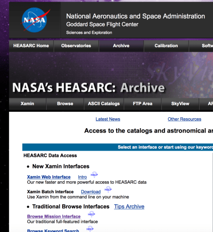
  • 数据下载,在 HEASARC 网站 Archive 目录下选中 Browse Mission Interface Screen Shot 2016-08-19 at 12.31.45 AM.png

我也不知道,这么无脑的东西,我截屏说明一下是为什么。我们直接到 RXTE 的 PCA 数据处理流程好了。

1.1 PCA 数据预处理

总体的思路是为了筛选出我们需要的数据文件,然后可通过 fasebin 以及 fbssum 折叠轮廓,或者使用得到的数据文件自己对数据处理得到脉冲轮廓。


$ heainit

$ xdf

点击  Reset -> 选中 FTP NO File -> 地址选择当前文件夹(.)或者填写绝对路径 -> 点击 Save -> 点击 Make ObsList

注意:点击 Make Obslist 显示申请观测号之前,不能选中 Time Range 或是 Subsystems 中的选项,否则会导致无法生成观测号。

点击 Make ObsList -> 在 Observation 中选中观测号 -> 选中 PCA -> 点击 Make AppIdConfigList -> 选择数据模式 -> 点击 Make FileList -> 输入保存的文件名 -> 点击 Save Filelist

指定目录下生成了提取出的对应观测号以及仪器下的数据文件(.xdf)。

$ maketime filename.xfl gti

通过给定的判据+过滤文件,筛选出数据的“好时间段”。其中过滤文件(.xfl)在 stdprod 中直接拷贝,判据(expression):elv.gt.10.and.offset.lt.0.02

在对单独的观测号处理时,判据没给出 pcu 的开关,默认 pcu 五个全开。在批处理(Rex)中会得到更加准确的 expression,包含了 pcu 信息。

$ fselect (.xdf中指定的文件) gtifilter_file “gtifilter(‘git’)”

通过好时间文件筛选出好时间数据。

$ fselect gtifilter_file fselect_file @bitfile

利用 bitfile 进一步筛选需要的时间文件

bitfile 的内容和格式:

以 crab 脉冲星 RXTE 96802-01-18-00 观测号为例:Screen Shot 2016-08-19 at 2.06.19 AM.png

Event == b1_ _ _ xxxxxxxxx 通过二进制编码表征一些标记,包括 M 标记事例是真事例还是时钟信号,{1} 表示占 1 位编码。D 标记 PCU 的开关情况,[0:4] 表征 ?{3} 占3位二进制码。C 是筛选能道,可以使用逻辑运算符选择能道区间。 E 标记探测器的阳极丝。


太阳系质心修正

$ faxbary fselect_file faxbary_file ./orbit/orbitfile ra=sourceRA dec=sourceDEC

由于关注的是源的周期性相关的物理信息,所以需要将光子到达探测器的时间,转换到到达太阳心质心的时间。否则光子信号会有一个与卫星的轨道以及地球的轨道有关的一个周期叠加。

生成质心修正后的示例型文件,至此,可以自行搜寻脉冲周期和折叠轮廓。


2. Python 搜寻周期折叠相

脉冲周期 f(t) 由 Taylor 多项式展开描述(不准确,离散的数据更准确的描述应该是差分多项式的 牛顿级数展开):

f(t) = f(t_0)+(t-t_0)f'(t_0)+\frac{(t-t_0)^2f''(t_0)}{2}

那么以t_0为时间零点,到达时间为t_i 的光子相位,由上式两边乘以(t-t_0)

\phi_i = (t_i-t_0)[f(t_0)+ \frac{(t_i-t_0)f'(t_0)}{1} + \frac{(t_i-t_0)^2f''(t_0)}{2}]

import numpy as np
import matplotlib.pyplot as plt
import pyfits as pf
import os
###########################
# read data from FITS file(optional)
# if this block is used, comment out next block then

#fpath = “/home/youli/Documents/crab_data/96802-01-21-00/faxbary_96802”
#hdulist = pf.open(fpath)

#tb = hdulist[1].data
#data = tb.field(2)

#hdulist.close()
###########################
# read data file from txt file
filename = ‘faxbary_0817_t1.txt’
data = np.loadtxt(filename)
##########################
# preset parameters
data = data – min(data)
N = len(data)
m = 100 # DOF for chi_square test
#nbin = 1000 # bin for histogram
b = N/m
f = np.arange(28.500,29.000,1e-2) # frequency searching range
chi_square = []

##########################

#search the best frequency utilizing the Chi-square test, where Chi-square is maxium

fbest = f[chi_square.index(max(chi_square))]

phi_tmp = np.mod(data*fbest,1.0)

p_num = np.histogram(phi_tmp,m)[0]

plt.figure(2)

p_num_x = np.arange(1.,m+1.,1)/m

#########################

# plot profile in 2 periods

#(if plot of 1 period is needed, comment out this block and use new commented block instead)

p_num_x_2_tmp = p_num_x + 1;p_num_x_2_tmp.tolist()

p_num_x_2 = p_num_x.tolist();p_num_2 = p_num.tolist()

p_num_x_2.extend(p_num_x_2_tmp);p_num_2.extend(p_num_2)

plt.plot(p_num_x_2,p_num_2)

#########################

#plot profile in one period

#plt.plot(p_num_x,p_num)

#########################

# print parameters

print “——————————–\n”,”INPUT PARAMETERS: \n”

print “input file: “,os.path.abspath(filename)

print “DOF of chi_square test: “,m

print “\nOUTPUT PARAMETERS: \n”

print “best frequency = “,fbest,”Hz”,”\nperiod = “,1/fbest,”s”

print “——————————–”

plt.show()

对自转频率的搜索利用的是 Chi-Square test。先计算光子的“相对相位”

\Phi_i = \frac{(t_i-t_0)}{T} mod 1.0

若信号不存在周期性,则光子的相位会呈现均匀分布

遇到的问题

LOG20160720

This is the first day I officially move in the lab. My boss assigned few papers for me to read.

  • The strongest cosmic magnets: Soft Gamma-ray Repeaters and Anomalous X-ray Pulsars
  • Magnetars: properties, origin and evolution
  • Formation of very strongly magnetized neutron stars: Implications for Gamma-ray bursts

the first two papers are review papers of magnetars, which is probably the first subject I will work on. The last paper is the first paper suggesting the existing of magnetars.

I spent whole afternoon deleting and reinstalling computer system. Ubuntu 15.10 was installed. But I was told that this version of Ubuntu wouldn’t upgrade anymore. Reinstalling of Ubuntu 16.4 is on the to-do list.

A tiny tip of reinstalling system: be sure to copy some important info of previous system, like DNS service, IP Address. Rookie mistake was made by me XD

你会解方程,你会写代码,你会调仪器,你会在学术报告上眉飞色舞。你是赢家。

我撸管,我抽烟,我宿醉,我在三平米的垃圾里骂社会主义。我是wanker