明早作报告,天呐,今晚又要加班了。记录下这两天学到的东西和工作
1. RXTE 数据处理流程
- 数据下载,在 HEASARC 网站 Archive 目录下选中 Browse Mission Interface

我也不知道,这么无脑的东西,我截屏说明一下是为什么。我们直接到 RXTE 的 PCA 数据处理流程好了。
1.1 PCA 数据预处理
总体的思路是为了筛选出我们需要的数据文件,然后可通过 fasebin 以及 fbssum 折叠轮廓,或者使用得到的数据文件自己对数据处理得到脉冲轮廓。
$ heainit
$ xdf
点击 Reset -> 选中 FTP NO File -> 地址选择当前文件夹(.)或者填写绝对路径 -> 点击 Save -> 点击 Make ObsList
注意:点击 Make Obslist 显示申请观测号之前,不能选中 Time Range 或是 Subsystems 中的选项,否则会导致无法生成观测号。
点击 Make ObsList -> 在 Observation 中选中观测号 -> 选中 PCA -> 点击 Make AppIdConfigList -> 选择数据模式 -> 点击 Make FileList -> 输入保存的文件名 -> 点击 Save Filelist
指定目录下生成了提取出的对应观测号以及仪器下的数据文件(.xdf)。
$ maketime filename.xfl gti
通过给定的判据+过滤文件,筛选出数据的“好时间段”。其中过滤文件(.xfl)在 stdprod 中直接拷贝,判据(expression):elv.gt.10.and.offset.lt.0.02
在对单独的观测号处理时,判据没给出 pcu 的开关,默认 pcu 五个全开。在批处理(Rex)中会得到更加准确的 expression,包含了 pcu 信息。
$ fselect (.xdf中指定的文件) gtifilter_file “gtifilter(‘git’)”
通过好时间文件筛选出好时间数据。
$ fselect gtifilter_file fselect_file @bitfile
利用 bitfile 进一步筛选需要的时间文件
bitfile 的内容和格式:
以 crab 脉冲星 RXTE 96802-01-18-00 观测号为例: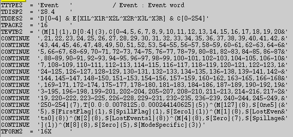
Event == b1_ _ _ xxxxxxxxx 通过二进制编码表征一些标记,包括 M 标记事例是真事例还是时钟信号,{1} 表示占 1 位编码。D 标记 PCU 的开关情况,[0:4] 表征 ?{3} 占3位二进制码。C 是筛选能道,可以使用逻辑运算符选择能道区间。 E 标记探测器的阳极丝。
太阳系质心修正
$ faxbary fselect_file faxbary_file ./orbit/orbitfile ra=sourceRA dec=sourceDEC
由于关注的是源的周期性相关的物理信息,所以需要将光子到达探测器的时间,转换到到达太阳心质心的时间。否则光子信号会有一个与卫星的轨道以及地球的轨道有关的一个周期叠加。
生成质心修正后的示例型文件,至此,可以自行搜寻脉冲周期和折叠轮廓。
2. Python 搜寻周期折叠相
脉冲周期  由 Taylor 多项式展开描述(不准确,离散的数据更准确的描述应该是差分多项式的 牛顿级数展开):

那么以 为时间零点,到达时间为
 的光子相位,由上式两边乘以
![\phi_i = (t_i-t_0)[f(t_0)+ \frac{(t_i-t_0)f'(t_0)}{1} + \frac{(t_i-t_0)^2f''(t_0)}{2}]](https://s0.wp.com/latex.php?latex=%5Cphi_i+%3D+%28t_i-t_0%29%5Bf%28t_0%29%2B+%5Cfrac%7B%28t_i-t_0%29f%27%28t_0%29%7D%7B1%7D+%2B+%5Cfrac%7B%28t_i-t_0%29%5E2f%27%27%28t_0%29%7D%7B2%7D%5D+&bg=ffffff&fg=333333&s=0&c=20201002)
import numpy as np
import matplotlib.pyplot as plt
import pyfits as pf
import os
###########################
# read data from FITS file(optional)
# if this block is used, comment out next block then
#fpath = “/home/youli/Documents/crab_data/96802-01-21-00/faxbary_96802”
#hdulist = pf.open(fpath)
#tb = hdulist[1].data
#data = tb.field(2)
#hdulist.close()
###########################
# read data file from txt file
filename = ‘faxbary_0817_t1.txt’
data = np.loadtxt(filename)
##########################
# preset parameters
data = data – min(data)
N = len(data)
m = 100 # DOF for chi_square test
#nbin = 1000 # bin for histogram
b = N/m
f = np.arange(28.500,29.000,1e-2) # frequency searching range
chi_square = []
##########################
#search the best frequency utilizing the Chi-square test, where Chi-square is maxium
fbest = f[chi_square.index(max(chi_square))]
phi_tmp = np.mod(data*fbest,1.0)
p_num = np.histogram(phi_tmp,m)[0]
plt.figure(2)
p_num_x = np.arange(1.,m+1.,1)/m
#########################
# plot profile in 2 periods
#(if plot of 1 period is needed, comment out this block and use new commented block instead)
p_num_x_2_tmp = p_num_x + 1;p_num_x_2_tmp.tolist()
p_num_x_2 = p_num_x.tolist();p_num_2 = p_num.tolist()
p_num_x_2.extend(p_num_x_2_tmp);p_num_2.extend(p_num_2)
plt.plot(p_num_x_2,p_num_2)
#########################
#plot profile in one period
#plt.plot(p_num_x,p_num)
#########################
# print parameters
print “——————————–\n”,”INPUT PARAMETERS: \n”
print “input file: “,os.path.abspath(filename)
print “DOF of chi_square test: “,m
print “\nOUTPUT PARAMETERS: \n”
print “best frequency = “,fbest,”Hz”,”\nperiod = “,1/fbest,”s”
print “——————————–”
plt.show()
对自转频率的搜索利用的是 Chi-Square test。先计算光子的“相对相位”

若信号不存在周期性,则光子的相位会呈现均匀分布
遇到的问题
 (真值也记为
 作为参数
作为参数  。
。 落入真值左右某个区间
 ![[\theta-\Delta\theta_2, \theta + \Delta\theta_1]](https://s0.wp.com/latex.php?latex=%5B%5Ctheta-%5CDelta%5Ctheta_2%2C+%5Ctheta+%2B+%5CDelta%5Ctheta_1%5D&bg=ffffff&fg=333333&s=0&c=20201002) 的概率为
的概率为  :
:
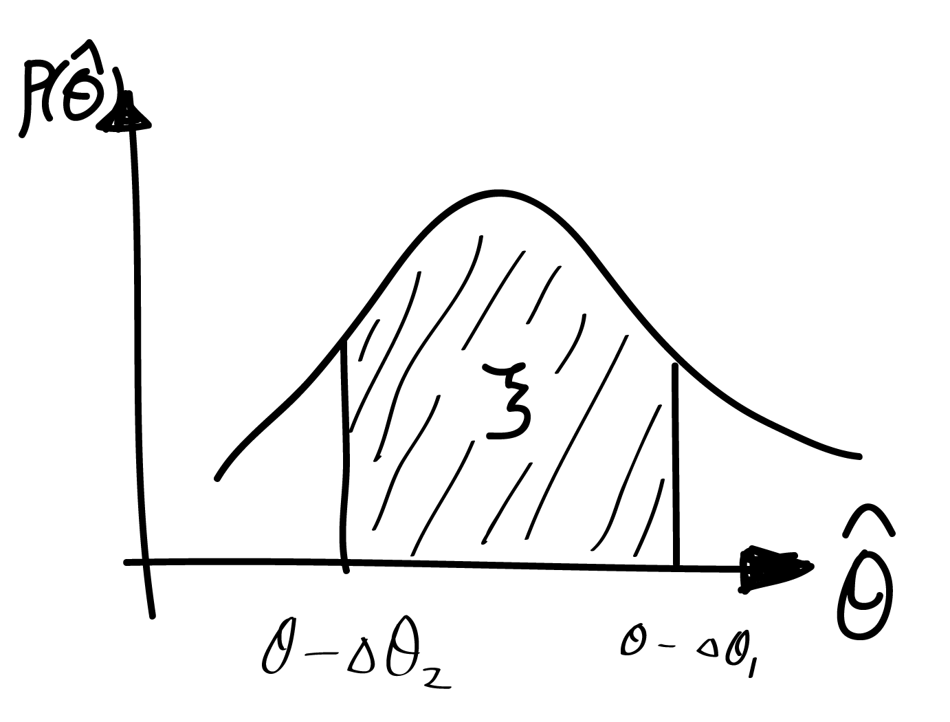

![[\hat{\theta} - \Delta\theta_1, \hat{\theta} + \Delta\theta_2 ]](https://s0.wp.com/latex.php?latex=%5B%5Chat%7B%5Ctheta%7D+-+%5CDelta%5Ctheta_1%2C+%5Chat%7B%5Ctheta%7D+%2B+%5CDelta%5Ctheta_2+%5D&bg=ffffff&fg=333333&s=0&c=20201002) 内,包含参数真值
内,包含参数真值 
 ,我们考虑样本的平均值的估计量。该样本的平均值是6。我们对这个样本进行bootstrap重采样,即以
 为样本空间,产生多组样本(这里产生5组)。我们对于重采样的样本
  将 参考样本
  则待估参量
则待估参量 ![[\hat{\theta}-\Delta\theta_1, \hat{\theta}+\Delta\theta_2]](https://s0.wp.com/latex.php?latex=%5B%5Chat%7B%5Ctheta%7D-%5CDelta%5Ctheta_1%2C+%5Chat%7B%5Ctheta%7D%2B%5CDelta%5Ctheta_2%5D&bg=ffffff&fg=333333&s=0&c=20201002) 。这里的待估参量则是真值,不是第一组参考样本的估计量,而这里的估计值则是第一组参考样本的估计量,所以
。这里的待估参量则是真值,不是第一组参考样本的估计量,而这里的估计值则是第一组参考样本的估计量,所以 (置信水平 60%)

![\frac{1}{4\pi} \nabla \cdot \vec{E} = - \frac{1}{4\pi} \nabla \cdot (\frac{\vec{\Omega}\times \vec{r} \times \vec{B}}{c}) = - \frac{1}{4\pi} \nabla \cdot [\frac{(\vec{\Omega}\times \vec{r}) \times \vec{B}}{c}]](https://s0.wp.com/latex.php?latex=%5Cfrac%7B1%7D%7B4%5Cpi%7D+%5Cnabla+%5Ccdot+%5Cvec%7BE%7D+%3D+-+%5Cfrac%7B1%7D%7B4%5Cpi%7D+%5Cnabla+%5Ccdot+%28%5Cfrac%7B%5Cvec%7B%5COmega%7D%5Ctimes+%5Cvec%7Br%7D+%5Ctimes+%5Cvec%7BB%7D%7D%7Bc%7D%29+%3D+-+%5Cfrac%7B1%7D%7B4%5Cpi%7D+%5Cnabla+%5Ccdot+%5B%5Cfrac%7B%28%5Cvec%7B%5COmega%7D%5Ctimes+%5Cvec%7Br%7D%29+%5Ctimes+%5Cvec%7BB%7D%7D%7Bc%7D%5D&bg=ffffff&fg=333333&s=0&c=20201002)
![\frac{1}{4\pi} \nabla \cdot \vec{E} = - \frac{1}{4\pi} \left\{ \vec{B} \cdot [ \nabla \times \frac{ \vec{\Omega} \times \vec{r}} {c}] - \frac{(\vec{\Omega}\times \vec{r})}{c} \cdot (\nabla \times \vec{B}) \right\}](https://s0.wp.com/latex.php?latex=%5Cfrac%7B1%7D%7B4%5Cpi%7D+%5Cnabla+%5Ccdot+%5Cvec%7BE%7D+%3D+-+%5Cfrac%7B1%7D%7B4%5Cpi%7D+%5Cleft%5C%7B+%5Cvec%7BB%7D+%5Ccdot+%5B+%5Cnabla+%5Ctimes+%5Cfrac%7B+%5Cvec%7B%5COmega%7D+%5Ctimes+%5Cvec%7Br%7D%7D+%7Bc%7D%5D+-+%5Cfrac%7B%28%5Cvec%7B%5COmega%7D%5Ctimes+%5Cvec%7Br%7D%29%7D%7Bc%7D+%5Ccdot+%28%5Cnabla+%5Ctimes+%5Cvec%7BB%7D%29+%5Cright%5C%7D&bg=ffffff&fg=333333&s=0&c=20201002)

![\frac{1}{4\pi} \nabla \cdot \vec{E} = - \frac{1}{4\pi} \left\{ \vec{B} \cdot [ \nabla \times \frac{ \vec{\Omega} \times \vec{r}} {c}] - (\frac{\Omega r \sin \theta}{c}\vec{\phi}) (\frac{\Omega r \sin \theta}{c}(\nabla \cdot \vec{E})\vec{\phi}) \right\}](https://s0.wp.com/latex.php?latex=%5Cfrac%7B1%7D%7B4%5Cpi%7D+%5Cnabla+%5Ccdot+%5Cvec%7BE%7D+%3D+-+%5Cfrac%7B1%7D%7B4%5Cpi%7D+%5Cleft%5C%7B+%5Cvec%7BB%7D+%5Ccdot+%5B+%5Cnabla+%5Ctimes+%5Cfrac%7B+%5Cvec%7B%5COmega%7D+%5Ctimes+%5Cvec%7Br%7D%7D+%7Bc%7D%5D+-+%28%5Cfrac%7B%5COmega+r+%5Csin+%5Ctheta%7D%7Bc%7D%5Cvec%7B%5Cphi%7D%29+%28%5Cfrac%7B%5COmega+r+%5Csin+%5Ctheta%7D%7Bc%7D%28%5Cnabla+%5Ccdot+%5Cvec%7BE%7D%29%5Cvec%7B%5Cphi%7D%29+%5Cright%5C%7D&bg=ffffff&fg=333333&s=0&c=20201002)
![[1-(\Omega r/c)^2 \sin^2 \theta] \frac{\nabla \cdot \vec{E} }{4 \pi} = - \frac{1}{4\pi} [\vec{B}\cdot(\nabla \times \frac{\Omega r \sin \theta}{c} \vec{\phi})]](https://s0.wp.com/latex.php?latex=%5B1-%28%5COmega+r%2Fc%29%5E2+%5Csin%5E2+%5Ctheta%5D+%5Cfrac%7B%5Cnabla+%5Ccdot+%5Cvec%7BE%7D+%7D%7B4+%5Cpi%7D+%3D+-+%5Cfrac%7B1%7D%7B4%5Cpi%7D+%5B%5Cvec%7BB%7D%5Ccdot%28%5Cnabla+%5Ctimes+%5Cfrac%7B%5COmega+r+%5Csin+%5Ctheta%7D%7Bc%7D+%5Cvec%7B%5Cphi%7D%29%5D&bg=ffffff&fg=333333&s=0&c=20201002)
 can be calculated by
  calculator as spherical coordinate form:
![\nabla \times \frac{\Omega r \sin \theta}{c} \vec{\phi} = \frac{1}{r \sin \theta}[\frac{ \partial}{\partial \theta}(\sin \theta \frac{\Omega r \sin \theta}{c})- \frac{\partial 0 }{\partial \phi}] \vec{e_r} + \frac{1}{r}[\sin \theta \frac{\partial 0 }{\partial \phi} - \frac{\partial}{\partial r} ( r \frac{\Omega r \sin \theta}{c})]\vec{e_{\theta}} + \frac{1}{r}[\frac{\partial}{\partial r}(r 0) - \frac{\partial 0 }{\partial \theta}] \vec{e_{\phi}}](https://s0.wp.com/latex.php?latex=%5Cnabla+%5Ctimes+%5Cfrac%7B%5COmega+r+%5Csin+%5Ctheta%7D%7Bc%7D+%5Cvec%7B%5Cphi%7D+%3D+%5Cfrac%7B1%7D%7Br+%5Csin+%5Ctheta%7D%5B%5Cfrac%7B+%5Cpartial%7D%7B%5Cpartial+%5Ctheta%7D%28%5Csin+%5Ctheta+%5Cfrac%7B%5COmega+r+%5Csin+%5Ctheta%7D%7Bc%7D%29-+%5Cfrac%7B%5Cpartial+0+%7D%7B%5Cpartial+%5Cphi%7D%5D+%5Cvec%7Be_r%7D+%2B+%5Cfrac%7B1%7D%7Br%7D%5B%5Csin+%5Ctheta+%5Cfrac%7B%5Cpartial+0+%7D%7B%5Cpartial+%5Cphi%7D+-+%5Cfrac%7B%5Cpartial%7D%7B%5Cpartial+r%7D+%28+r+%5Cfrac%7B%5COmega+r+%5Csin+%5Ctheta%7D%7Bc%7D%29%5D%5Cvec%7Be_%7B%5Ctheta%7D%7D+%2B+%5Cfrac%7B1%7D%7Br%7D%5B%5Cfrac%7B%5Cpartial%7D%7B%5Cpartial+r%7D%28r+0%29+-+%5Cfrac%7B%5Cpartial+0+%7D%7B%5Cpartial+%5Ctheta%7D%5D+%5Cvec%7Be_%7B%5Cphi%7D%7D+&bg=ffffff&fg=333333&s=0&c=20201002)


![[1-(\Omega r/c)^2 \sin^2 \theta] \rho = - \frac{1}{4 \pi}(\vec{B} \cdot \frac{2}{c}\vec{\Omega})](https://s0.wp.com/latex.php?latex=%5B1-%28%5COmega+r%2Fc%29%5E2+%5Csin%5E2+%5Ctheta%5D+%5Crho+%3D+-+%5Cfrac%7B1%7D%7B4+%5Cpi%7D%28%5Cvec%7BB%7D+%5Ccdot+%5Cfrac%7B2%7D%7Bc%7D%5Cvec%7B%5COmega%7D%29+&bg=ffffff&fg=333333&s=0&c=20201002)