Abstract: HXMT, Hard X-ray Modulation Telescope is the project I’ve been working on. The major purpose in this period is to calculation the energy flux of instruments on satellite. My last work log introduced the numerical calculation tool of my work, Mathematica, which maybe not as elegant and cool as what c++ or python does, but it turns out that works at all. This log mainly focused on the relevant physics stuff concerned in this work, which contained spectral model of astro-sources, interstellar absorption model, effective area of instrument.
RADIATIVE PROCESSES IN ASTROPHYSICS
As my last log mentioned, approximately half of my work first focused on the INTEGRAL catalog. obviously, the first thing before calculating the HXMT energy flux is verify the method and spectral model are trustworthy. Well, the INTEGRAL provided the general reference catalog, of which I used version 39. In the catalog, there are 4 columns reported the value of calibration energy flux calculated by XSPEC. (It’s a good idea to post some logs of XSPEC) So, the first step is to calculate the flux in 10-50KeV, 20-60KeV, 60-200KeV with the model parameters given by the site: http://isdc.unige.ch/integral/catalog/39/catalog.html The reported calibration value are given in unit of cgs, so the energy fluxes are in unit of 


those two equation calculated the powerlaw model and cutoff model, in which A refers to normalization coefficient and 
INTERSTELLAR ABSORPTION
In the content above I didn’t mention that calibration value includes a energy range 3-10KeV, in which energy range the photon is call soft X-ray radiation. The extragalactic radiation of X-ray is dominated by soft X-ray radiation. As the interstellar molecule have the property to absorb the radiation, the soft X-ray radiation must consider interstellar absorption effect.

where
there are many version of cross section, but INTEGRAL catalog utilizes Wisconsin Cross-section:

and the coefficients of analytic fit to cross section are given in following table:
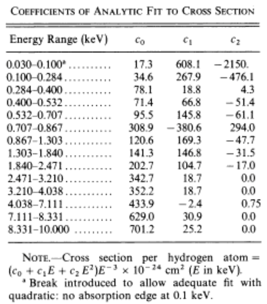
As we can see, the interstellar absorption only happened under the energy of 10KeV. So we can transfer the integration to the following form:

Though this log was aimed to introduce the physics regime, but it occurred to me to verifying the reason that Mathematica results had the deviation to XSPEC while considering the interstellar absorption which you have to carry out the numerical integration. So I utilized Python to set a parameter, energy bin, which is the same thing to interval. This parameter partitions the flux range to N sub-intervals.
and here’s the python code:
import numpy as np
import pylab as pl
import scipy
A=10 #normalization coefficient
nh=0.26 #column density of hydrogen(unit of 10**22atom/cm**2)
c=2.1 #photon index
N=20000 #energy bin=N
x1=np.linspace(3,3.21,N,endpoint=False)
y1=np.trapz(np.e**(-(342.7+18.7*x1+0*(x1**2))*(x1**(-3))*(10**(-24))*nh)*A/(6.24*(10**8))*x1*(x1**(-c)),x1)
x2=np.linspace(3.21,4.038,N,endpoint=False)
y2=np.trapz(np.e**(-(352.2+18.7*x2+0*(x2**2))*(x2**(-3))*(10**(-24))*nh)*A/(6.24*(10**8))*x2*(x2**(-c)),x2)
x3=np.linspace(4.038,7.111,N,endpoint=False)
y3=np.trapz(np.e**(-(433.9+(-2.4)*x3+0.75*(x3**2))*(x3**(-3))*(10**(-24))*nh)*A/(6.24*(10**8))*x3*(x3**(-c)),x3)
x4=np.linspace(7.111,8.331,N,endpoint=False)
y4=np.trapz(np.e**(-(629+30.9*x4+0*(x4**2))*(x4**(-3))*(10**(-24))*nh)*A/(6.24*(10**8))*x4*(x4**(-c)),x4)
x5=np.linspace(8.331,10,N,endpoint=False)
y5=np.trapz(np.e**(-(701.2+25.2*x5+0*(x5**2))*(x5**(-3))*(10**(-24))*nh)*A/(6.24*(10**8))*x5*(x5**(-c)),x5)
flux=y1+y2+y3+y4+y5 #unit of erg/cm^2/s
print flux
It turns out that XSPEC utilizes 

INSTRUMENT EFFECTIVE AREA
Instruments have different matrix responses for different photons in various energy. Till now we have considered the interstellar absorption, spectral and here’s another parameter we should integrate with, that is instrument effective area.

where D is observed value, F is the spectrum we knew, P is the matrix responses. For flux we care about, we can calculate the integration:

Those three aspects are in priority list of my recent work, I’ve introduce the basic physics behind it. For more information of HXMT, please visit the site: www.hxmt.cn
